Tissue composition and structure shape its electrical response. Pass a very small alternating current through muscle, fat or nerve, measure the voltage it produces, and the relationship between the two reflects what the tissue is made of and how it is built. This explainer covers the physics behind that idea, the standard model used to describe it, and how measurement conditions shape its interpretation.
Impedance, in plain terms
For a steady current, the relationship between voltage and current is resistance, as in Ohm’s law. With an alternating current, a material can also store and release charge during each cycle, so voltage and current no longer rise and fall together. Impedance captures both effects at once.
It is reported in one of two equivalent ways. The first splits it into resistance, the part in step with the current, which comes from ions drifting through fluid and dissipating energy, and reactance, the part a quarter-cycle out of step, which comes from charge being stored and released. The second gives a magnitude, how strongly the material opposes the current overall, and a phase angle, how far the voltage lags or leads the current. In tissue the reactance is capacitive, so the phase is negative: the current runs slightly ahead of the voltage.
Admittance is the inverse of impedance. It is often the more natural choice for tissue, because current divides between parallel paths, around cells and through them, and the admittances of parallel paths simply add. Physicists usually go one step further and describe the material itself by its conductivity and permittivity, which do not depend on the size or spacing of the electrodes. A measured impedance always mixes those material properties with the geometry of the measurement, a point taken up in Measuring at the point of contact.
Why frequency changes the answer
A cell is a conductive interior wrapped in a membrane only a few nanometers thick. The membrane is a lipid layer that barely lets ions through, so it behaves much like a capacitor: two conductors separated by a thin insulator. Between cells lies extracellular fluid, a salt solution that conducts well.Reference 1Reference 2
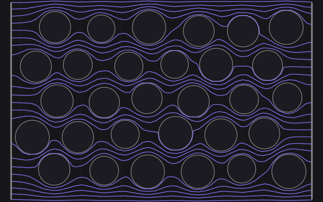
At low frequencies each membrane has time to charge fully during every cycle and then blocks further current, so current flows around cells through the extracellular fluid. As frequency rises the membranes have less time to charge, their reactance falls, and current increasingly crosses them and uses the cell interiors as well. More conducting paths means lower impedance. Figure 1 shows the two regimes side by side.
a Low frequency
b High frequency

- Current paths, equal current between neighboring lines
- Cell bounded by its membrane
- Electrodes at either side
The shift from “around” to “through” is called the beta dispersion: the band of frequencies where membrane charging dominates the response. Herman Schwan’s classic work described three main dispersion regions in tissue, and later surveys, measurements and models spanning a very wide frequency range built on that picture.Reference 1Reference 3Reference 4
- Alpha dispersion
- The lowest frequencies, roughly hertz to kilohertz. Associated with ionic effects around charged cell surfaces and membrane structures. In practice this is also where electrode effects are largest, which makes it the hardest region to measure cleanly.
- Beta dispersion
- Roughly kilohertz to tens of megahertz. Charging of cell membranes and other internal interfaces. The region most closely tied to cell size, shape and packing.
- Gamma dispersion
- Gigahertz frequencies. Rotation of water molecules, which mainly reflects how much water the tissue holds.Reference 6
The boundaries are approximate and the regions overlap. Gabriel and colleagues needed several overlapping dispersion terms to describe tissue spectra from 10 Hz to 100 GHz.Reference 5
The Cole model, in words
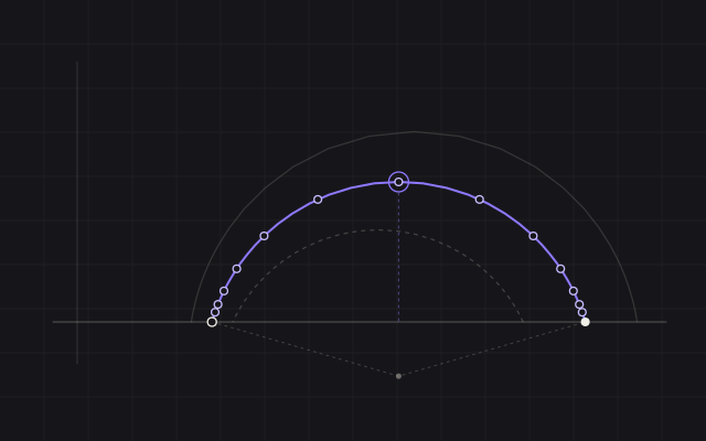
In 1941 the brothers Kenneth and Robert Cole showed that the dielectric response of many materials traces a circular arc when plotted in the complex plane, with the center of the arc sitting below the axis.Reference 7 A closely related expression for impedance, usually called the Cole model, became the standard way to describe a single tissue dispersion.Reference 8
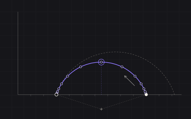
It needs four numbers. R0 is the resistance at the low-frequency limit of this dispersion, where current travels mainly through the fluid around cells. R∞ is the resistance at the high-frequency limit of this dispersion, where membranes no longer block current and the paths inside and outside cells act in parallel. The characteristic frequency marks the middle of the transition, where the reactance is largest. A fourth, dimensionless exponent, also written α but unrelated to the alpha dispersion, completes the set. A single ideal relaxation time gives a semicircle. A broader distribution of relaxation times produces a depressed arc; the fitted exponent describes that spread. Each Cole term describes one transition; real tissue spectra contain overlapping dispersions, so wide-band tissue models combine several terms.Reference 5
a Impedance plane: reactance against resistance
b Across frequency, low to high
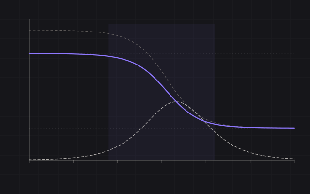
- Cole model (a: the arc; b: magnitude)
- Points at evenly spaced log frequencies; frequency rises from right to left along the arc
- R0, low-frequency limit
- R∞, high-frequency limit
- Characteristic frequency, top of the arc
- Phase, shown as the size of the negative angle
- Same model with a higher R0, as with less extracellular fluid
- Transition band
The model is useful because it compresses a whole spectrum into a few interpretable numbers, and it fits many tissue measurements well.Reference 9 It is still a description, not an explanation. A good fit does not prove a particular mechanism, different combinations of parameters can produce similar curves over a limited frequency range, and some measurements do not follow it at all: in one study of human liver at microwave frequencies, the ex vivo data could be described by a Cole–Cole fit while the in vivo data could not.Reference 10
What shapes a tissue’s spectrum
Because the beta dispersion comes from current negotiating membranes, anything that changes the amount, shape or arrangement of those membranes, or the fluid around them, changes the spectrum.
- Cell size, shape and packing. Densely packed cells leave narrow extracellular channels and raise the low-frequency resistance. Larger cells take longer to charge, which moves the transition toward lower frequencies.
- Extracellular fluid. More fluid between cells lowers R0. Cell swelling, which squeezes the space between cells, raises it.
- Membrane integrity. Damaged membranes stop blocking current, which flattens the dispersion.
- Orientation. Skeletal muscle conducts differently along and across its fibers, particularly at lower frequencies. Epstein and Foster studied this directional dependence in skeletal muscle.Reference 11
- Fat and water. Adipose tissue is mostly large lipid-filled cells with little water and conducts poorly; tissues rich in water and electrolytes conduct well. Literature surveys show wide differences across tissue types.Reference 2Reference 3
This is why differences between tissues are physically plausible. A peripheral nerve is a bundle of long, oriented fibers wrapped in connective tissue and often fat. Muscle is a dense array of long cells. Fat is mostly lipid. A vessel wall is layered and carries blood. Structures this different have every reason to respond differently to current. Distinguishing them reliably under surgical conditions, at the point of contact, is an open research question.
What confounds the picture
The same properties that make tissue spectra informative also make them sensitive to conditions that have nothing to do with tissue type.
- Temperature. Ionic conduction increases with temperature, so the same tissue reads differently at room and body temperature. Careful studies state the temperature of every measurement.Reference 9
- Hydration and surface fluid. Exposed tissue dries out. Blood, irrigation saline and tissue fluid add conductive layers that can carry current along the surface instead of through the tissue.
- Time after excision. Once blood supply stops, cells change. In excised swine liver, resistivity rose over the first two hours and then fell; the authors suggested the fall reflected membrane breakdown.Reference 12 Living, perfused tissue and excised tissue are not interchangeable.Reference 10
- Variation between specimens. Age, species, anatomical site, disease and handling all move spectra. Differences between two specimens of the same tissue can rival differences between tissue types.
- The measurement itself. Electrode effects, contact area and pressure, and cabling all leave their mark, particularly at low frequencies. They are the subject of the next insight.
In practice
Interpreting a tissue spectrum
Impedance reports the bulk electrical behavior of the volume the current passes through. Three points govern how a spectrum is read.
- The spectra of different tissues overlap, and one tissue varies with conditions. A single-frequency reading alone does not establish reliable tissue identification.
- The volume a measurement reflects depends on electrode size, spacing and contact. At a boundary between tissues, it mixes them.
- Turning a spectrum into a statement about tissue takes reference data, a defined method and an evaluation that holds up on new specimens. Evaluating tissue-sensing data covers what that involves.
References
Schwan HP. Electrical properties of tissue and cell suspensions. Advances in Biological and Medical Physics. 1957;5:147–209. doi:10.1016/b978-1-4832-3111-2.50008-0 · PMID 13520431
Foster KR, Schwan HP. Dielectric properties of tissues and biological materials: a critical review. Critical Reviews in Biomedical Engineering. 1989;17(1):25–104. PMID 2651001
Gabriel C, Gabriel S, Corthout E. The dielectric properties of biological tissues: I. Literature survey. Physics in Medicine and Biology. 1996;41(11):2231–2249. doi:10.1088/0031-9155/41/11/001 · PMID 8938024
Gabriel S, Lau RW, Gabriel C. The dielectric properties of biological tissues: II. Measurements in the frequency range 10 Hz to 20 GHz. Physics in Medicine and Biology. 1996;41(11):2251–2269. doi:10.1088/0031-9155/41/11/002 · PMID 8938025
Gabriel S, Lau RW, Gabriel C. The dielectric properties of biological tissues: III. Parametric models for the dielectric spectrum of tissues. Physics in Medicine and Biology. 1996;41(11):2271–2293. doi:10.1088/0031-9155/41/11/003 · PMID 8938026
Schwan HP, Foster KR. Microwave dielectric properties of tissue: some comments on the rotational mobility of tissue water. Biophysical Journal. 1977;17(2):193–197. doi:10.1016/S0006-3495(77)85637-3 · PMID 836937
Cole KS, Cole RH. Dispersion and absorption in dielectrics I. Alternating current characteristics. The Journal of Chemical Physics. 1941;9(4):341–351. doi:10.1063/1.1750906
Grimnes S, Martinsen ØG. Bioimpedance and Bioelectricity Basics. 3rd ed. Academic Press; 2015. ISBN 978-0-12-411470-8.
Stoy RD, Foster KR, Schwan HP. Dielectric properties of mammalian tissues from 0.1 to 100 MHz: a summary of recent data. Physics in Medicine and Biology. 1982;27(4):501–513. doi:10.1088/0031-9155/27/4/002 · PMID 7089048
O’Rourke AP, Lazebnik M, Bertram JM, et al. Dielectric properties of human normal, malignant and cirrhotic liver tissue: in vivo and ex vivo measurements from 0.5 to 20 GHz using a precision open-ended coaxial probe. Physics in Medicine and Biology. 2007;52(15):4707–4719. doi:10.1088/0031-9155/52/15/022 · PMID 17634659
Epstein BR, Foster KR. Anisotropy in the dielectric properties of skeletal muscle. Medical & Biological Engineering & Computing. 1983;21(1):51–55. doi:10.1007/BF02446406 · PMID 6865513
Haemmerich D, Ozkan R, Tungjitkusolmun S, et al. Changes in electrical resistivity of swine liver after occlusion and postmortem. Medical & Biological Engineering & Computing. 2002;40(1):29–33. doi:10.1007/BF02347692 · PMID 11954705

